
Q-Learning Implementation
This page covers the technical implementation of the original agent design, an episodic Q-learning agent with an epsilon-greedy policy
Background
When I began working on the agent implementation, I had not yet learned about continuous task agents, average reward, and soft policies. Thus, when I was determining the best algorithm to use for this problem, I arrived at Q-learning with an epsilon-greedy policy. Now, in hindsight as I write this page, some of these choices were naive, but I was not yet aware of more advanced agent options better suited for this problem, or how to formulate problems in the continuous task setting. The purpose of this page is to highlight the choice that was made, show what happened with that choice and some tweaking, and then show how we arrive at the softmax actor-critic design with average reward.
Q-Learning and Expected SARSA
When I was deciding on a temporal difference (TD) method, I was ultimately choosing between Q-learning and Expected SARSA. Both of these would use the same epsilon greedy policy, but there’s a key difference in the value functions here:
Q-learning action-value update function

Expected SARSA action-value update function

In the Q-learning action-value update, the agent is very “optimistic” and its value for the next state only considers the best possible action taken in the next state. In the Expected SARSA update, the agent considers all of the possible outcomes of the next state weighted by their probability of occurring based on the policy. Since the policy is epsilon-greedy, the weights are 1-epsilon for the action with max Q value and epsilon for all other actions.
Let me highlight this difference in the example of a grid world with a cliff:

Image from Adrian Yijie Xu on https://medium.com/gradientcrescent/fundamentals-of-reinforcement-learning-navigating-cliffworld-with-sarsa-and-q-learning-cc3c36eb5830
The agent always starts at S and tries to get to G in the shortest amount of time possible. In each square, the agent can go up, down, left, or right. Going in a direction which would place the agent outside of the grid world border results in the agent remaining in the same state; however, if the agent goes into the cliff, it receives a -100 reward and the episode ends. At all other times, the agent receives a -1 reward to encourage it to reach G in as few steps as possible.
A Q-learning agent learns to take the red path. Most of the time it doesn’t end up going over the cliff, but at any square next to the cliff the agent has an epsilon probability of going over the cliff
An Expected SARSA agent learns to take a path more like the blue one, where it provides itself a buffer knowing that there is always a probability of going over the cliff if it stays next to it.
Why is this? Let’s say that epsilon is 0.05 (meaning that 5% of the time the agent will randomly select the non-greedy action). Advancing into a square adjacent to the cliff then has very different values for the Q-learning and Expected SARSA agent:
Q-learning: -1 (best outcome)
Expected SARSA: 3 x (.95 x -1) for no fall action, 1 x (0.05 x -100) for the fall action = -5.15
(Now, these of course aren’t exact as there is a discount factor as well as the factoring in of remaining steps to the end of the episode, but it conveys the idea: being near the cliff is a much worse state for the Expected SARSA agent than the Q-learning agent)
Q-Learning Choice & Problem Formulation
Considering that our energy optimization problem doesn’t have any inherent “risks” like falling off of a cliff, we really want to take all the “risk” we can to get the most energy. Thus, we don’t need any protection mechanism like an Expected SARSA agent has for adverse actions, and Q-learning is the better choice for this problem over Expected SARSA.
So, to define our agent and the reward function:
Q-learning agent
Epsilon greedy policy
Reward = power measured by solar panel at given motor positions
Episodic task
Q-Learning Agent Performance Examples
So, without further ado, how did the agent perform in this problem?
Initial Agent Parameters:
exp_step_size = 0.1 # agent step size
exp_epsilon = 0.1 # epsilon value for exploration
exp_discount_factor = 0 # discount value (naively tried to simulate non-episodic)
exp_initialization_value = 0.05 # initialization value of the action-values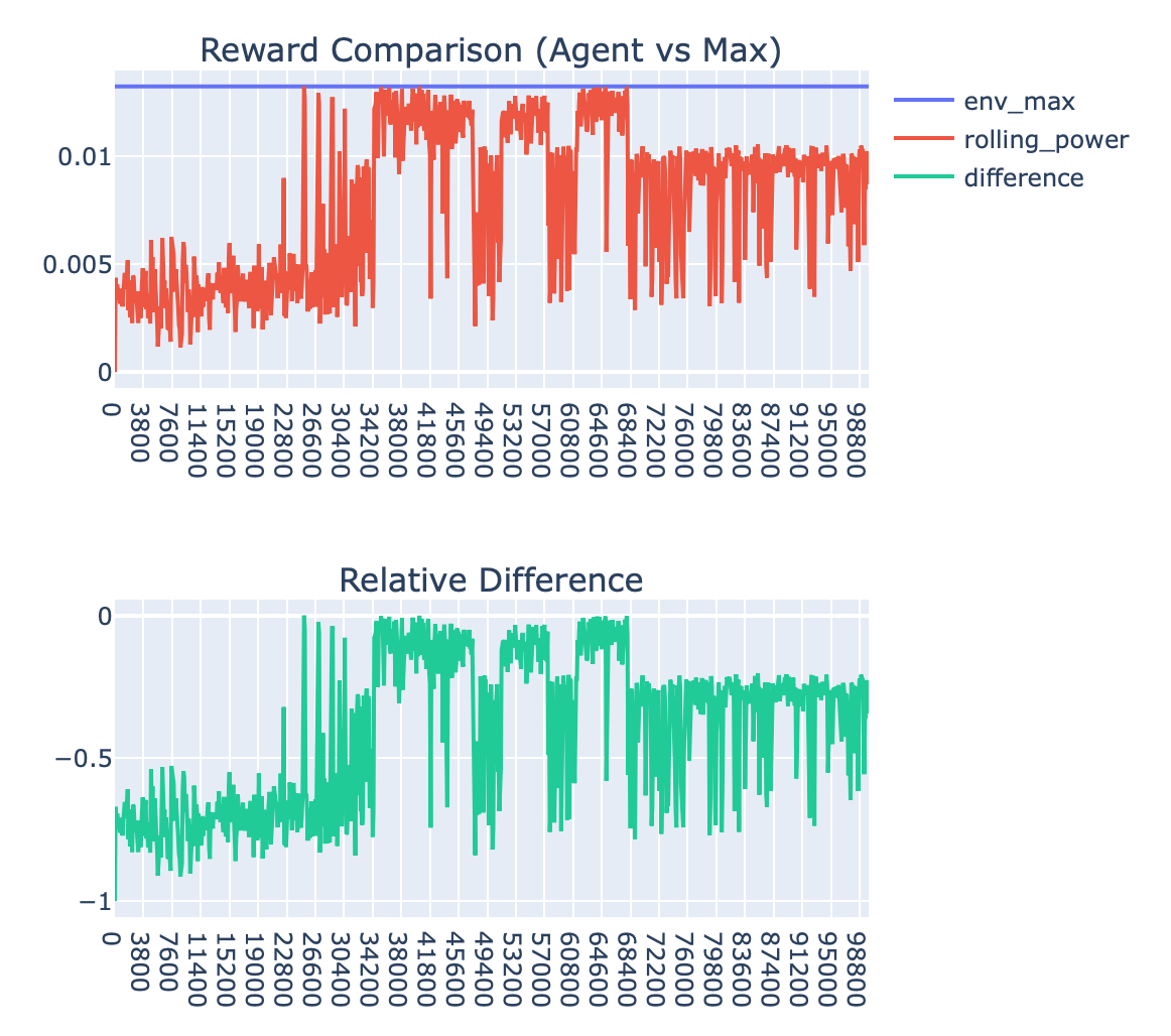
Performance Review
The agent intermittently finds the optimal state, but has significant deviations from the optimal state due to the nature of the policy
After 64,000 steps, the agent appears to have settled on some suboptimal state and does not return to the true optimal state
The agent takes around 30,000 steps to get to the optimal state with some stability, which is quite long and indicative that the agent is probably not performing very well
I played around with the step size parameter and saw the best behavior for a value of 0.09:

This still has some potential convergence issues and takes over 26k steps to make any significant learning progress. Why does it take so long? My first theory was that the agent is simply not landing upon the optimal index for a while, after which it then jumps around that vicinity. To remedy this I increased epsilon (to 0.2) to try and get the agent to explore more. This produced worse results as the agent is exploring too much now and not spending enough time at the optimal state:

Based on this, I tried shrinking epsilon to see what would happen (to 0.01) and saw a big improvement in stability once optimum had been reached, but the persistent issue of taking a very long time to reach optimum.

At this point, I needed to take a new approach to root-causing this performance issue of slow discovery of the optimal state. I created a visualization to observe the frequency with which the agency was visiting each state and noticed something really interesting: The agent was visiting states with roughly the same distribution as the magnitude of their power values.
Now, one the one hand, this means that the agent has learned the environment well
On the other hand, this is not optimal. The agent is unnecessarily spending too much time in suboptimal states. The agent state visit frequency shouldn’t match the environments reward — it should be disproportionally visiting good states over bad states.

Figure 1: Number of times the agent had visited each state by step 24,000 in the experiment
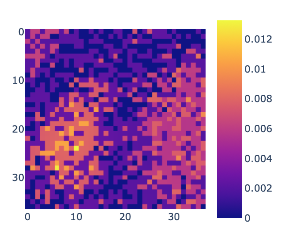
Figure 2: The environment reward for each state
Based on this finding, I tried a variety of things related to:
action-value initializations (setting to 0, to the avg of env return, and to a value well above max env return all to no avail)
action-value update function changes (to try and account for visitation bias I was seeing, to no avail)
Everything above the line was prior to taking Course 3 and 4 of the RL Specialization on Coursera (see Helpful RL Resources). It became clear that there were some larger conceptual issues with the approach I was taking for this problem, and I paused work on the agent to go back and continue the RL Specialization series I was in. This shed so much light on the problem after learning about policy gradient methods and continuous task (average reward) settings.
Q-Learning Agent Shortcomings
So, with this newly acquired RL knowledge, I could see that the Q-learning agent had a few critical shortcomings for this problem:
this task is inherently continuous, not episodic, so the temporal difference (TD) updates had poor value updates given the episodic “intention”
I was setting discount factor to 0 to try and accommodate for this
If I was simply training the agent to reach the optimal index (like completing a maze), this would work as an episodic task; however, I am trying to get the agent to continuously produce the most energy, and that optimal index will change as lighting conditions change
slow learning, as the agent was taking around 20,000 steps to identify an optimal solution, and would not remain there
the policy was epsilon-greedy and had suboptimal exploration, as any time it wasn’t doing the greedy action it was exploring the others (whether how good or how bad it knew them to be) with equal probability
Let’s visualize that last point. Consider the below image, which is trying to show the action values for three example states.

In a Q-learning agent, the action-values and policy are inherently tied together. For each state above, say that the the curvy looking lines are trying to represent the action value for all the possible actions in a given state. We could identify the best, second best, third best, . . ., and nth best action.
The rectangular shapes overlaid on each state are representing the probability with which a given action is chosen:
the highest valued action in each state has a 1 - epsilon probability of being chosen
all other actions—regardless of how they are ranked—have an epsilon probability of being chosen
Do we see how this could be problematic for optimizing total energy? When exploring, the agent is equally likely to explore both the worst action and second best action. Let’s visualize this.

Greedy Agent: In each of the three states, the agent happens to select the greedy action (which it does with probability 1 - epsilon)
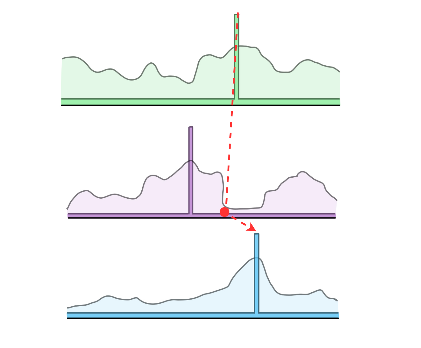
Suboptimal Exploration: In state 2, the agent has selected a non-greedy action. It has epsilon probability of exploring, and then 1/N probability of selecting each action — regardless of their expected value (where N is the number of actions - 1)
On the left, we see a sequence of three state transitions in which the agent’s policy has selected the greedy action each time. On the right, we see a sequence where the agent selects one of the worst actions in the second state, then the greedy action in the third state.
The Need for an Improved Agent
Based on all the information above, it’s clear we need a new approach for the agent design.
How do we decouple action selection from action values?
How can we explore more intelligently?
How should we adapt to the continuous nature of this problem?
How can we arrive at the optimal state earlier?
Theoretically we could use a decaying epsilon value, however this does not generalize well to other problems and would face issues as the lighting environment changes and the optimal index moves around. See how these are addressed at the sequel to this page, RL Agent - Softmax Actor-Critic
