Experiment Design
This page details the generation of data for a simulated environment, and how we can assess agent performance based on this data
Overview
To develop our RL algorithm, we want to have a simulation environment that the agent can interact with faster than if it was interacting with a real environment. This lets us learn about our agent faster, make tweaks, and build a better agent — which we can then deploy to the real physical system once we’re confident in our algorithm choice.
This page covers that development process in detail, going over:
experiment design
generating simulation data
benchmarking performance in the simulation environment
Experiment Design
How do we ultimately know that the RL agent works nominally? To create a sandbox for validating the RL agent, let’s simplify the problem into a two phases:
The lighting is stationary — can the RL agent discover the optimal position to be in?
The lighting is non-stationary (like the real world) — does the RL reasonably adjust itself to optimize energy produced over some time window?
We ideally want to have a confident solution to case 1 before moving onto the more challenging case 2. So, how do we produce realistic simulated data for our agent to use?
Generating Simulation Data
The general process is below:
Force the solar panel to scan the entire state space
With the values returned (power at each motor position), we now have our states and values of those states

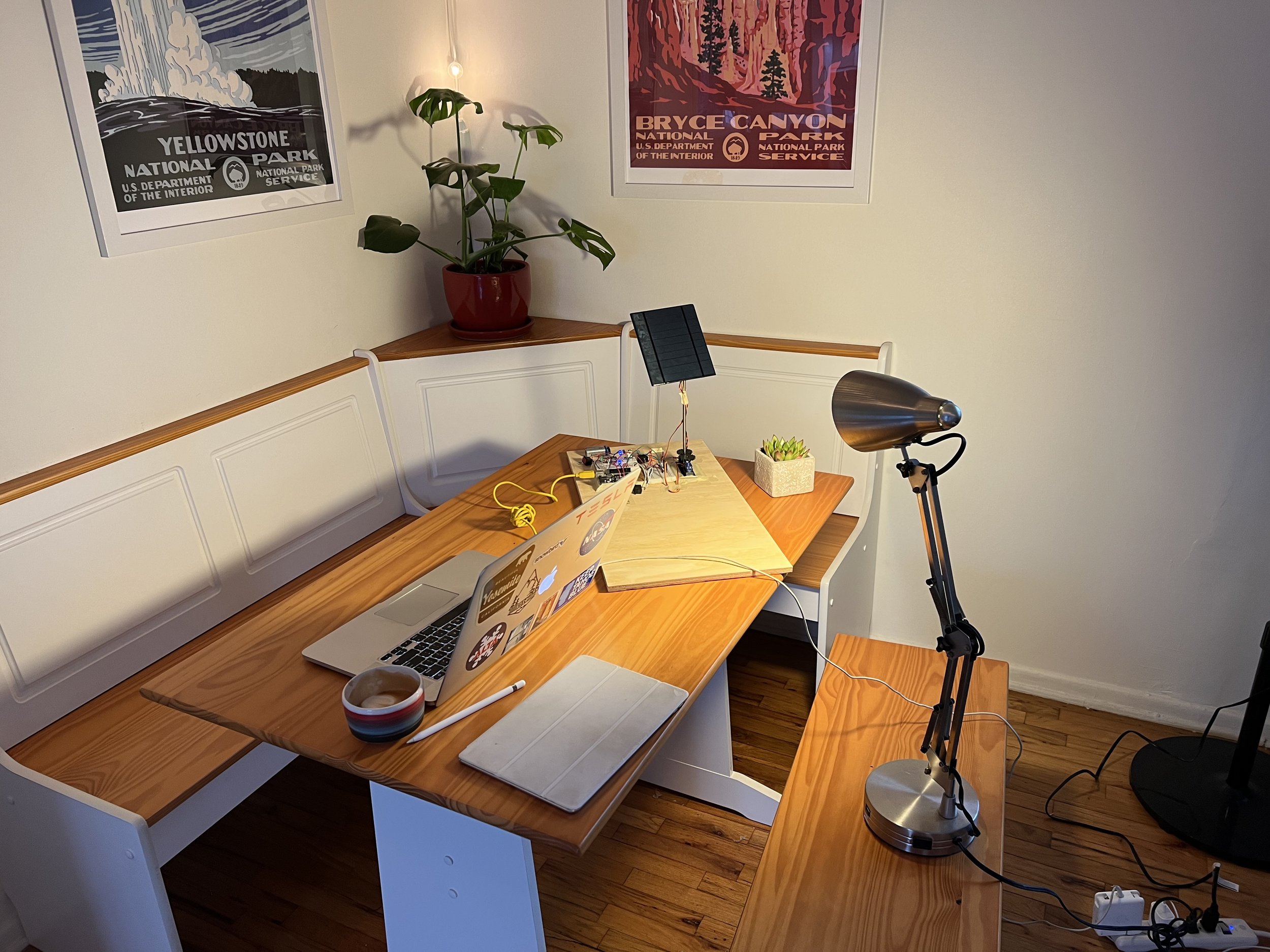
In real-life, this looks like:


In this particular scan, the lamp did not produce a very noticeable effect (it’s just an LED bulb), and the nearby windows had diffuse, weak light from a cloudy day. The next day I took a scan with the panel directly in front of a window, which produced a more defined optimum panel position


In the graph on the left, we see more defined contours from the scan. Rotating the graph to view it as more of a 2D histogram, we can see that the panel was optimal positioned with motor 1 between 120-140 degrees and motor 2 between 0-60 degrees.
Now, each of the motor indices here go from 0-180. Knowing the physical limitations of the gears in the hardware design, there is not much discrepancy at 1 degree increments, so I map the index positions by a scaling factor of 5. Thus, we end up with a index range of (0/5, 180/5) —> (0, 36) and a grid that’s 37x37.
Benchmarking Performance in the Simulated Environment
Plotting the 2D histogram of power at each index position:

We see that the max value is at the index of (24, 10). Thus, we would expect that an agent in a static environment would learn to be in position (24,10) most frequently. This is our objective assessment of agent performance, where we can compare the power that an agent would have generated if it were in the optimal position the entire time vs the power the agent actually generates.
To visualize this, here’s an example performance assessment from the Q-learning agent that was developed:
Blue shows the reward (power) the agent could have produced had it been in the (24,10) index above
Red shows the rolling avg of power generated by the agent
Green shows the relative difference between the optimal power at a given step and the power generated by the agent

The above is certainly not optimal performance. Shortcomings of this example agent are discussed on the Q-learning agent page, and the evolution of that agent is discussed on the Softmax Actor-Critic agent page.

