Optimizing Solar Energy Production with Reinforcement Learning
Jack O’Grady
April 28th, 2022
This research demonstrates a model-free approach to optimize the energy produced by a dual-axis solar panel using reinforcement learning. Specifically, a softmax actor-critic agent optimizes energy production in a simulated, dynamic lighting environment which is generated from real power data. All schematics, algorithms, and code are provided as open-source materials.
Introduction
Photovoltaic solar is playing a key role in the world’s transition to renewable energy, making up 46% of all new electric capacity added to the U.S. grid in 2021 [1]. While primary factors driving optimal panel positioning are readily modeled (i.e., the sun’s position at each time of day), site-specific and panel-specific factors are less so. Elements like dynamic shading from nearby trees or structures, localized panel defects, drift in axis positions as systems degrade, etc. can have significant impacts on energy production. Rather than modeling, calibrating, and updating all of these factors for each dual-axis solar installation, this research seeks to demonstrate how an AI agent employing reinforcement learning (RL) can optimize energy production without directly knowing any of these factors.
Controlling Systems with RL
RL is a paradigm shift in how we model and control complex systems. The designers of an RL agent neither need to model the dynamics of the system being controlled, nor do they need to understand how to control for each of these dynamics. In our solar energy optimization problem, our objective is to maximize energy production from the panel. To do that, optimal behavior would entail positioning the panel to generate the most power at any point of time during the day as the environment (lighting) changes.
Using traditional methods, we would take a development approach like the below, where we try to model each factor that affects the energy production of the system then develop control logic to account for each of those factors. We try different things, tune our controls and models, and ultimately attempt to reach optimal behavior.
For RL, the development approach is quite different—we simply define our objective, and the RL agent learns how to achieve optimal behavior for the problem without the designers of the RL agent having to know how to do so. The RL agent is either directly or indirectly learning the underlying dynamics of the system and responding optimally to each situation it finds itself in.
At a high level, the agent learns via the following process:
The agent interacts with the environment and receives some reward
The agent learns from the reward by updating its likelihood of selecting actions in a given state
The process repeats
With this background, we now discuss the specific RL implementation for our energy optimization problem.
For those interested, you can find more in-depth pages about reinforcement learning concepts on the following pages:
RL Fundamentals | Helpful RL Resources
RL Implementation
We first review the hardware of the system we are optimizing, then discuss the software and algorithms.
Dual-Axis Panel
In our problem, we have a dual-axis solar panel that we are trying to maximize the energy output of. Each axis is operated by a servo motor, which can rotate 180°, and the panel is able to measure the power produced for each position that it is in. At each time step, it broadcasts the motor positions and power being produced to the RL agent via serial communication over a USB port. Below, you can see a blueprint compared to the actual panel hardware.
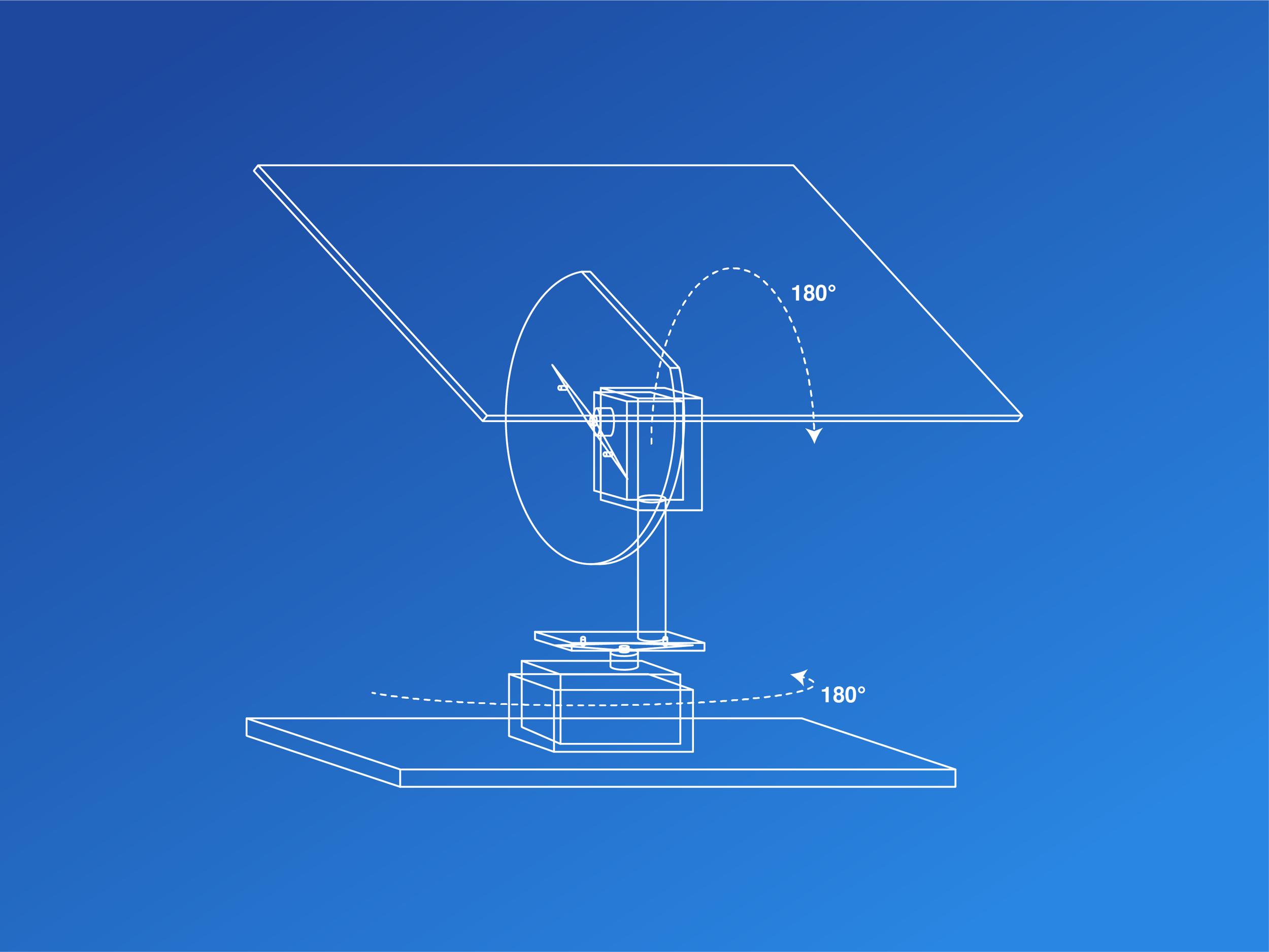
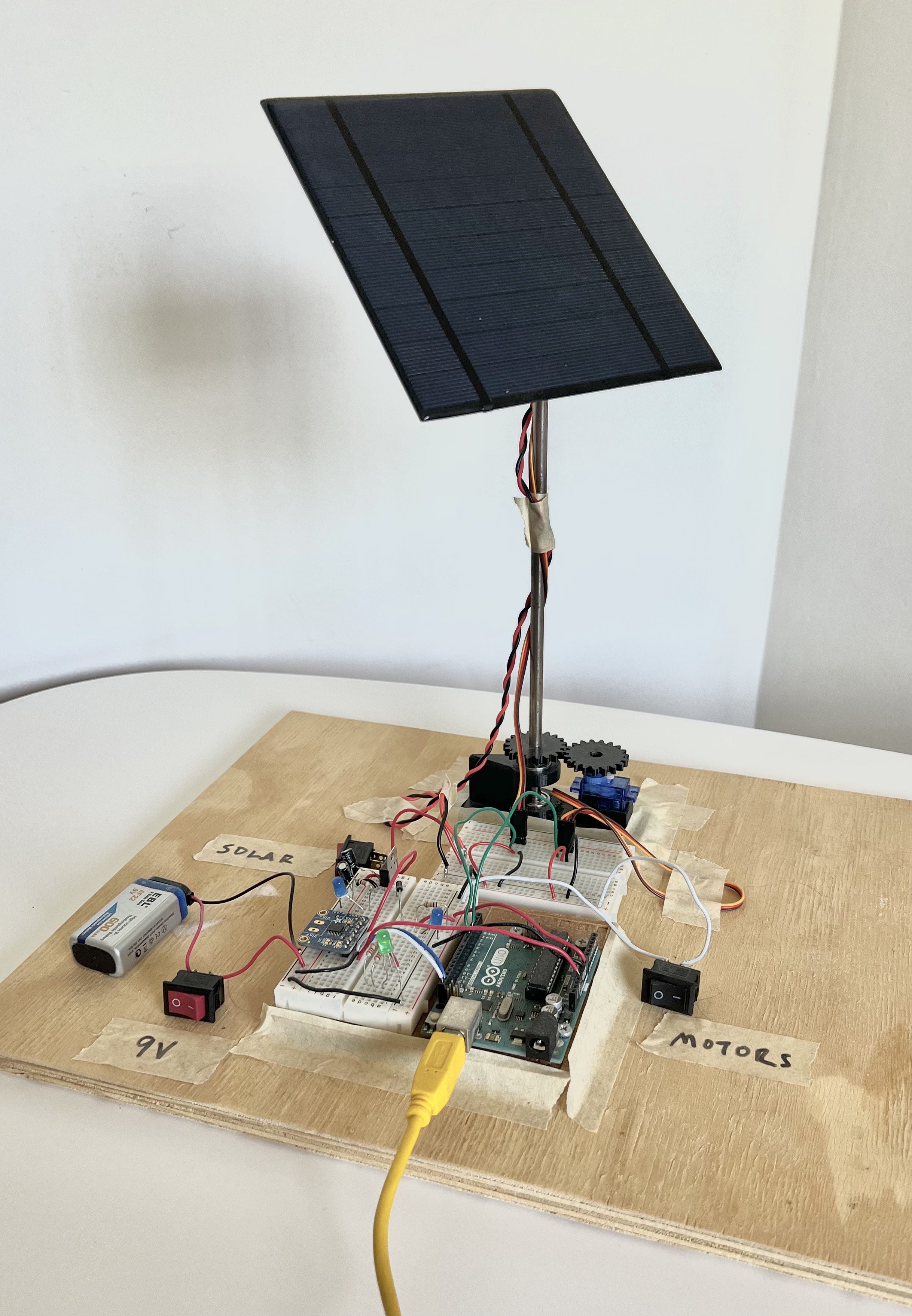
Detailed view of the dual-axis panel hardware
For those interested, you can find more detailed material on the dual-axis panel design on the following pages:
System Design | Circuit Schematic | Dual-Axis Panel Design
Agent-Environment Interaction
At each time step, the agent must decide how the motors should be positioned to produce the most energy. Each motor can be positioned from 0-180°, but the 3D printed gears used in this project only allow about 5° of precision in panel positioning. To account for this, I map the 0-180° positions to indices of 5° increments. This means that each motor can be in position 0 to 36. To simplify the agent’s memory structure, we convert the 2D index of motor position (say [36, 1]) into a flat mapped 1D index position (say [1333]), which conveys the state of both motors with a single index.
In addition to the motor positions, as the environment shifts throughout the day, the agent also tracks time of day as part of its state. There is a configurable time-of-day partition value which can increase or decrease the discretization of distinct states the agent learns, but in this implementation it is set to 24 to map to each hour of the day.

The agent interacts with the environment by requesting motor index positions, then learns from the power produced at those indices at that time of day
This is the nexus of the information the agent has and the actions that it can take to optimize energy. We now discuss how the agent uses this information to achieve that objective.
Agent Design
The agent in this optimization problem employs a softmax actor-critic algorithm with tabular representations of the actor and critic networks. I chose this implementation after initially experimenting with a Q-learning agent using an epsilon-greedy policy, which had difficulty efficiently exploring the large action space (of which there are 1369 actions in any state). Given the continuous nature of this task, our actor and critic update equations also use average reward rather than a discount factor and future state values.
The agent’s update equations are shown below:

Delta equation for our agent

Actor update equation for our agent. See RL Agent - Softmax Actor-Critic for details on this gradient simplification.

Critic update equation for our agent
In each state, the agent must select which motor position index to transition to next, one of which corresponds to staying in the same position. When the agent makes its decision, the environment transitions the panel positions and returns reward, which is the amount of power produced in the new state less some energy required to rotate the motors. In the graphic below, we visualize how the agent is selecting which action to take:
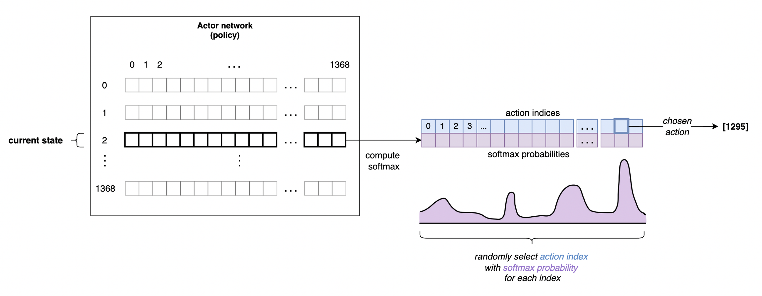
A visualization of how the actor’s learned values of each action influence its probability of being selected in a softmax policy
The actor and critic networks are three dimensional and of size [time of day partitions, number of states, number of actions]. In this implementation, that equates to a size of [24, 1369, 1369]. The values inside of the actor network correspond not to the actual power expected in each state, but rather the probability with which that action should be selected. The critic has a similar three-dimensional memory structure; however, it is learning the expected power from each action given the state.
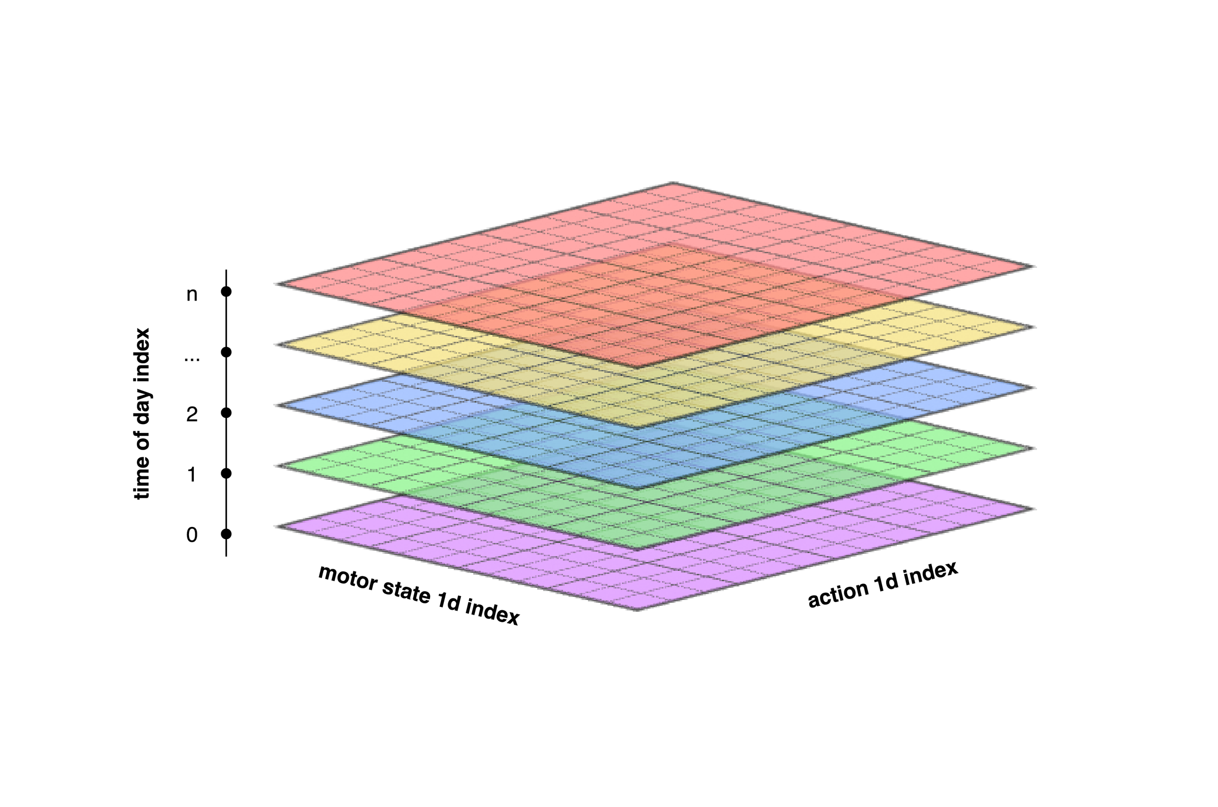
A visualization of the three-dimensional structure of the actor and critic networks
With the agent design covered, we now transition to the training environment in which the agent learns optimal behavior.
For those interested, you can find more detailed, technical pages on agent implementations in this project at the following links:
RL Agent - Softmax Actor-Critic | RL Agent - Q-Learning
Generating Simulated Environments
RL agents learn from exploration, and exploration takes time. We typically navigate this in RL by using simulated environments wherein one step of simulation time is significantly shorter than one step of real time. This allows us to quickly learn whether or not a given agent implementation is well-suited for a problem, as well as conduct a hyperparameter study.
In this problem, since we do not want to model all the underlying dynamics that affect real power generation in a given place at a given time, we generate a simulated environment from a real light-scan using the dual-axis panel. This is done using the following high-level process:

Visually, this looks like:
Collect power measurement at all motor indices
The above is a timelapse capture, not real-time
Convert to 2D array

The light scan from the video above in 3D

The light scan from the video above as the 2D reward array passed to the environment class
Add to environment class
The environment class emulates the dynamic lighting environment that the agent will actually face in deployment by both shifting the array every N steps (sun moving in the sky), and resetting it to its initial position every M steps (days). N and M are currently set to 3,600 and 86,400, respectively, to represent the seconds in an hour and in a day. Thus, in our simulation 3,600 steps corresponds to 1 hour of real time, and 86,400 steps corresponds to 1 day of real time.
The environment class also internally adds a power draw penalty for moving the motors. For testing the agent, it’s fairly arbitrary how accurate the motor power draw per angle is—we just want to have some penalty for the agent moving the motors so it has to learn how to balance exploration (which consumes motor power) with exploitation (staying in the current position and not drawing current for the motors).
Thus, the environment’s reward is:

Where the motor power draw is defined as:

Sigma is defined as some constant. In this implementation, sigma is set to 0.0001W per degree of movement per motor
For those interested, you can find more detailed, technical pages on the environment and simulation generation at the following links:
Experiment Design | Experiment I: Shifting Env | Experiment II: Shifting Env with Time of Day
Results
I first conduct a hyperparameter study by sweeping the agent’s temperature, actor step size, critic step size, and average reward step size from 1e-5 to 1e0 in 10x increments, which leads to 625 permutations of agent hyperparameters. In the simulation for the hyperparameter study, I use 1M steps and assess performance based on the rolling average of power generation at the end of the simulation.
Based on this study, the below hyperparameter set was determined to be the most performant:
temperature: 0.001actor_step_size: 1.0critic_step_size: 0.1avg_reward_step_size: 1.0
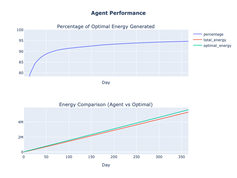
To understand the performance of our system, we simulate one year’s worth of data and assess the energy produced by the agent as compared to the energy that would have been generated if the panel was perfectly positioned at each time step. Since we’re using 1 simulation step = 1 second, we need 365 * 86,400 = 31,536,000 simulation steps. Running this, we get the following agent performance:
Within 1 month of operation, our agent is producing over 90% of the true optimal energy each day—all without needing any models or human inputs to capture and control for the environment dynamics. As the year goes on, the agent continues to learn and improve its energy production, achieving 96% of true optimal energy per day by the end of the year.
Examining agent behavior at the beginning of the simulation, we can see how the agent explores many actions the first time it encounters each state, then starts to narrow down its action selections as the hours go on. Below, we visualize the first 5 days of operation by hour:
Comparing the rolling power that the agent generates for the first million steps versus the last million steps, we also see how the agent’s behavior converges to optimal while the agent continues to learn.
To further validate agent performance, we pass in a different light scan and use the same agent algorithm and hyperparameters. This light scan has much more defined regions of high power and lower power states:

A separate light scan with more pronounced peaks and troughs.

The 2D reward array based on the light scan.
Running the simulation for 31,536,000 steps (a year in simulation), the agent again achieves around 95% of true optimal energy per day by the end of the year.
Conclusion
This research demonstrates that a softmax actor-critic agent can optimize energy production for a dual-axis solar panel with a completely model-free, domain-knowledge-free approach. The agent optimizes for power generation, handles multiple dynamic lightning environments, and, in simulations emulating a year of operation, consistently achieves 95% of the fully optimal energy production per day.
While traditional methods and domain knowledge could theoretically model and solve an optimization problem like this, they don’t necessarily scale as the number of panels in an installation grows (consider inter-panel shading dynamics), nor are the solutions applicable to other problems we face in our transition to renewable energy. This contrast between domain-knowledge-based methods and AI-based methods points to a larger question:
As we face an increasing number of engineering challenges with the world’s transition to renewable energy, how can we scale humanity’s problem-solving capability?
I believe that RL enables us to solve a greater number of optimal-control problems for complex energy systems in less time, with less human effort, and more optimally so than traditional, non-AI based methods.
Open-Source Project Materials
All schematics, algorithms, and code that went into this project are provided as open-source materials:
For detailed, technical content about each phase of the project, head to: Project Overview
To access the code used in this project, head to: Code Repository on Github
Future Directions
While I won’t be developing this research further, I see three promising future directions for it:
Update the Q-Network and Policy Network to Deep Neural Networks: By getting rid of tabular state and action representations, the agent becomes much more general and could be easily adapted to control multiple panels.
Multi-Panel Control: Utilize the underlying agent algorithm to control multiple panels, wherein certain panel positions shade the other panels in the solar array.
Convert the Agent to C/C++ for Standalone, Online Deployment: While the agent as is can technically be operated as an online agent, it requires having a laptop running Python connected to the Arduino. By porting the code to C/C++, the agent could be flashed onto the Arduino and run as a standalone, online agent whenever the Arduino is powered on.
References
[1] https://www.seia.org/solar-industry-research-data
© 2022 Jack O’Grady. All rights reserved.